Laminar flow & Turbulent Flow
- Laminar flow is the flow which occurs in the form of lamina or layers with no intermixing between the layers.
- Laminar flow is also referred to as streamline or viscous flow.
- In case of turbulent flow there is continuous inter mixing of fluid particles.
Reynold’s Number:
- The dimensionless Reynolds number plays a prominent role in foreseeing the patterns in a fluid’s behaviour. It is referred to as Re, is used to determine whether the fluid flow is laminar or turbulent.
Reynold’s no, Re
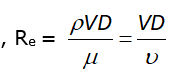
V=mean velocity of flow in pipe
D = Characteristic length of the geometry
μ = dynamic viscosity of the liquid (N – s /m2)
ν = Kinematic viscosity of the liquid (m2/s)
Where,
Ac = Cross – section area of the pipe
P = Perimeter of the pipe
Pipe | Plate |
Re < 2000 laminar 2000 < Re < 4000 Transient Re > 4000 turbulent | Re < 5 × 10⁵ Laminar Re > 5 × 10⁵ turbulent [transient is small so neglected] |
Case–I
Laminar flow in a pipe
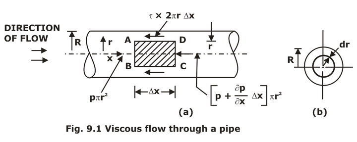
Now, forces acting on the fluid element are:
(a). The pressure force, P×πR2 of face AB.
(b). The pressure force on face CD. =
(c). The shear force, τ × 2πr∆x on the surface of fluid element. As there is no acceleration hence:
Net force in the x direction =0
ΣFx = 0 results in
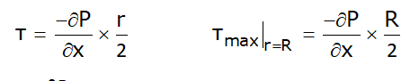
As ∂P/∂x across a section is constant, thus the shear stress τ varies linearly with the radius r as shown in the Figure.
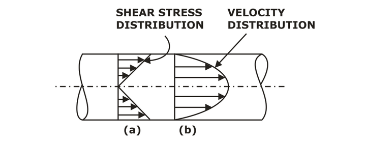
Shear stress and velocity distribution in laminar flow through a pipe
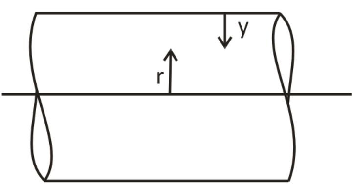
r + y = R
dr + dy = 0
dr = − dy
u =0 at r = R
Thus,
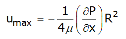
& u =uMax at r = 0
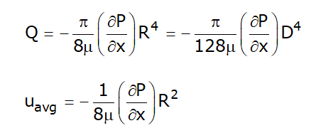
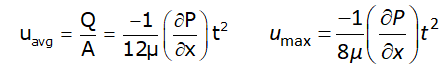
Discharge, Q = A × uavg
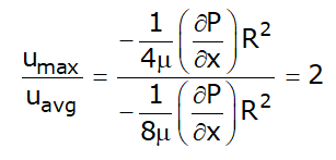
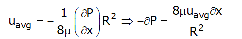
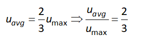
Ratio of maximum velocity to average velocity
Thus, Average velocity for Laminar flow through a pipe is half of the maximum velocity of the fluid which occurs at the centre of the pipe.
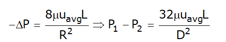
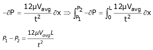
Pressure variation in Laminar flow through a pipe over length L
On integrating the above equation on both sides:
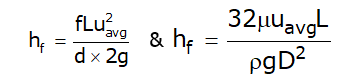
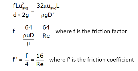
Head loss in Laminar flow through a pipe over length L
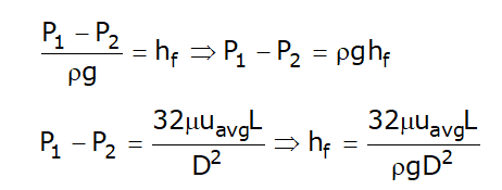
Above equation is hagen poiseuille equation.
As we know,
Thus,
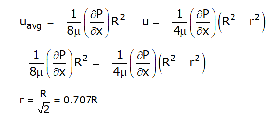
Radial distance from the pipe axis at which the velocity equals the average velocity
LAMINAR FLOW BETWEEN TWO FIXED PARALLEL PLATES
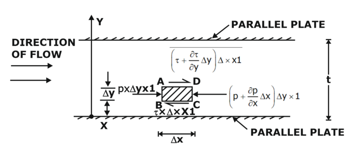
For steady and uniform flow, there is no acceleration and hence the resultant force in the direction of flow is zero.
![]()
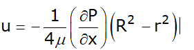
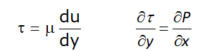
Velocity Distribution (u):
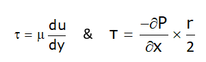
the value of shear stress is given by:
Boundary condition, at y = 0 u = 0
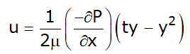
Thus, velocity varies parabolically as we move in y-direction as shown in Figure.
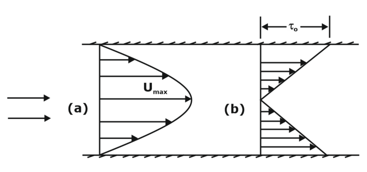
Velocity and shear stress profile for turbulent flow
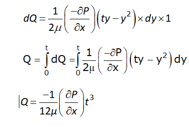
Discharge (Q) between two parallel fixed plates:
The average velocity is obtained by dividing the discharge (Q) across the section by the area of the section t ×1.
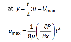
Ratio of Maximum velocity to average velocity:
Thus,
Pressure difference between two parallel fixed plates
CORRECTION FACTORS
There are two correction factors:
- Momentum correction factor (β)
- Kinetic energy correction factor (α)
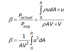
5.1. Momentum correction factor (β)
It is defined as the ratio of momentum per second based on actual velocity to the momentum per second based on average velocity across a section. It is denoted by β.
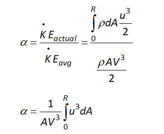
5.2. Kinetic energy correction factor (α):
It is defined as the ratio of kinetic energy of flow per second based on actual velocity to the kinetic energy of the flow per second based on average velocity across a same section.
Let p = momentum
P = momentum/sec.
5.3. For flow through pipes values of α and β:
Correction-factor | Laminar | Turbulent |
α | 2 | 1.33 |
β | 1.33 | 1.2 |
- From the above we can that the value of correction factor for Laminar flow is more than that for turbulent flow.
Turbulent flow
Turbulent flow is a flow regime characterized by the following points as given below
Shear stress in turbulent flow
In case of turbulent flow there is huge order intermission fluid particles and due to this, various properties of the fluid are going to change with space and time.
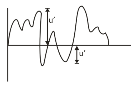
Average velocity and fluctuating velocity in turbulent flow
Boussinesq Hypothesis:
Similar to the expression for viscous shear, J. Boussinesq expressed the turbulent shear mathematical form as
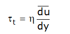
where τt = shear stress due to turbulence
η = eddy viscosity
u bar = average velocity at a distance y from boundary. The ratio of η (eddy viscosity) and (mass density) is known as kinematic eddy viscosity and is denoted by ϵ (epsilon). Mathematically it is written as

If the shear stress due to viscous flow is also considered, then …. shear stress becomes as
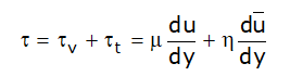
The value of η = 0 for laminar flow.
Reynolds Expression for Turbulent Shear Stress.
Reynolds developed an expression for turbulent shear stress between two layers of a fluid at a small distance apart, which is given as:
![]()
where u’, v’ = fluctuating component of velocity in the direction of x and y due to turbulence.
As u’ and v’ are varying and hence τ will also vary.
Hence to find the shear stress, the time average on both the sides of the equation
![]()
The turbulent shear stress given by above equation is known as Reynold stress.
Prandtl Mixing length theory:
According to Prandtl, the mixing length l, is that distance between two layers in the transverse direction such that the lumps of fluid particles from one layer could reach the other layer and the particles are mixed in the other layer in such a way that the momentum of the particles in the direction of x is same.
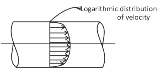
VELOCITY DISTRIBUTION IN TURBULENT FLOW
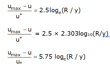
In above equation, the difference between the maximum velocity umax, and local velocity u at any point i.e. (umax - u) is known as ‘velocity defect’.
Velocity distribution in turbulent flow through a pipe
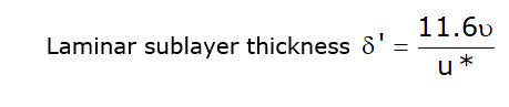
Laminar sublayer thickness


No comments:
Post a Comment
Knowing brings controversy