unsteady heat conduction

If the temperature of a body does not vary with time, it is said to be in steady state. But if there is an abrupt change in its surface temperature, it attains an equilibrium temperature or a steady state after some period. During this period, the temperature varies with time and body is said to be in the unsteady or transient state. This phenomenon is known as Unsteady or transient heat conduction.

Lumped System Analysis 

• Interior temperatures of some bodies remain essentially uniform at all times during a heat transfer process.
• The temperature of such bodies is only a function of time, T = T(t).
• The heat transfer analysis based on this idealization is called lumped system analysis.

Consider a body of the arbitrary shape of mass m, volume V, surface area A, density ρ and specific heat C_p initially at a uniform temperature T_i.  

• At time t = 0, the body is placed into a medium at temperature T_∞ (T_∞ >T_i) with a heat transfer coefficient h.  An  energy  balance  of  the  solid  for  a  time  interval  dt  can  be  expressed as:
  heat transfer into the body  during dt =  the increase in the energy of  the body during dt 
  h A (T_∞ – T) dt = m C_p dT 
• With m = ρV and change of variable dT = d(T – T_∞):
   
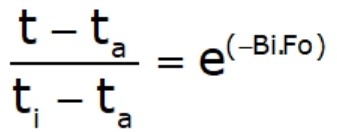
• Integrating from t = 0 to T = T_i
  

• Using above equation, we can determine the temperature T(t) of a body at time t, or alternatively, the time t required for the temperature to reach a specified value T(t). 
  Note that the temperature of a body approaches the ambient temperature T_∞ exponentially.

• A large value of b indicates that the body will approach the environment temperature in a  short time.  
• b is proportional to the surface area but inversely proportional to the mass and the specific heat of the body.
• The total amount of heat transfer between a body and its surroundings over a time  interval is:  Q = m C_p [T(t) – Ti]  The behavior of lumped systems can be interpreted as a thermal time  constant as shown in fig. below:

       

             

• Where R_t is the resistance to convection heat transfer and C_t is the lumped thermal capacitance of the solid. Any increase in R_t or C_t will cause a solid to respond more slowly to changes in its thermal environment and will increase the time respond required to reach thermal equilibrium. 
  

Criterion for Lumped System Analysis

• Lumped system approximation provides a great convenience in heat transfer analysis.We want to establish a criterion for the applicability of the lumped system analysis. A characteristic length scale is defined as: 
  L_c= V/A
• A nondimensional parameter, the Biot number, is defined: 
  

• The  Biot number is the ratio of the internal resistance  (conduction)  to the external resistance to heat convection.
• Lumped system analysis assumes a uniform temperature distribution throughout the body, which implies that the conduction heat resistance is zero. Thus, the lumped system analysis is exact when Bi = 0.
• It is generally accepted that the lumped system analysis is applicable if: Bi≤ 0.1
• Therefore, small bodies with high thermal conductivity are good candidates for lumped system analysis.  Note that assuming h to be constant and uniform is an approximation

Fourier number:
Fourier number is given by:

 

• The temperature of a body in the unsteady state can be calculated at any time only when Biot number < 0.1.

Characteristic Length: Characteristic length is denoted by l_c.

Characteristic Length for different Section

Transient Conduction in Large Plane Walls, Long Cylinders, and Spheres

• The lumped system approximation can be used for small bodies of highly conductive materials.
• But, in general, the temperature is a function of position as well as time.  
• Consider a plane wall of thickness 2L, a long cylinder of radius r₀, and a sphere of radius r₀ initially at a uniform temperature T_i

       

• We also assume a  constant heat transfer coefficient h  and neglect radiation. The formulation of the one‐dimensional transient temperature distribution T(x,t) results in a  partial differential equation (PDE), which can be solved using advanced mathematical methods. For the plane wall, the solution involves several parameters: 
  T = T (x, L, k, α, h, T_i, T_∞) 
  where α = k/ρC_p. 

• By using dimensional groups,we can reduce the number of parameters.
  Θ=Θ(x, Bi,τ)
• To find the temperature solution for plane wall, i.e. Cartesian coordinate, we should solve  the Laplace’s equation with boundary and initial conditions: 
  
  
  So, we can write: 
  
  where,